Forward Kinematics of a 2-Link Planar Manipulator

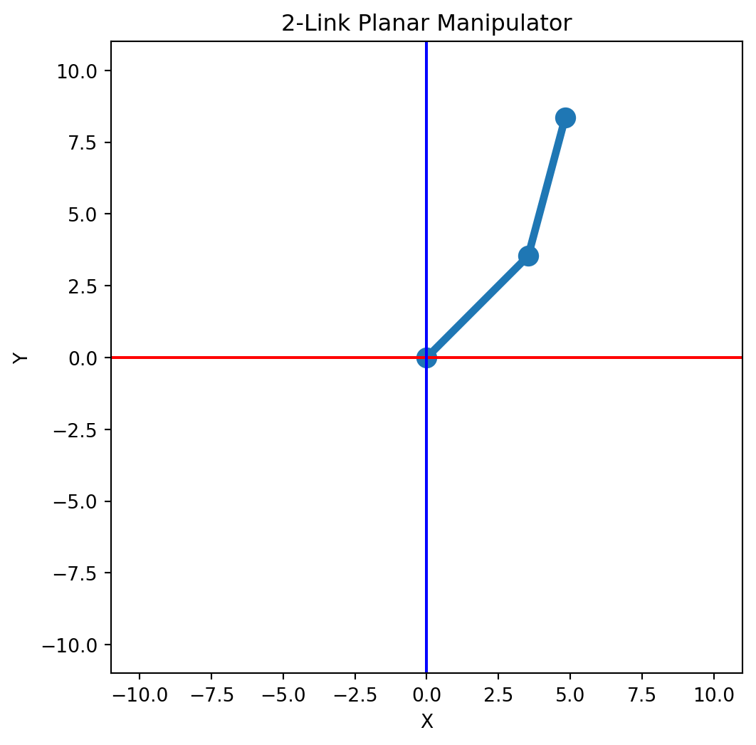
Simulating Forward Kinematics of 2-Link Planar Manipulator using Python

This article demonstrates the forward kinematics of a two-link planar robotic manipulator. Forward kinematics involves determining the position and orientation of the end-effector given the joint variables and link parameters.

To describe the kinematic structure of the manipulator, we use the Denavit–Hartenberg (DH) convention, which represents the spatial relationship between successive coordinate frames using four parameters: joint angle \(\theta_i\), link offset \(d_i\), link length \(a_i\), and link twist \(\alpha_i\).

---

Denavit–Hartenberg Transformation Matrix

Using the standard DH convention, the homogeneous transformation matrix that relates frame \(i\) to frame \(i-1\) is given by:

\[ {}^{i-1}_{i}T = \begin{bmatrix} \cos\theta_i & -\sin\theta_i\cos\alpha_i & \sin\theta_i\sin\alpha_i & a_i\cos\theta_i \\ \sin\theta_i & \cos\theta_i\cos\alpha_i & -\cos\theta_i\sin\alpha_i & a_i\sin\theta_i \\ 0 & \sin\alpha_i & \cos\alpha_i & d_i \\ 0 & 0 & 0 & 1 \end{bmatrix} \]

This matrix incorporates both the rotation and translation between two consecutive links of the manipulator (also knows as screw motion).

---

Overall Forward Kinematics

For a manipulator with \(n\) links, the transformation matrix that relates the end-effector frame \(n\) to the base frame \(0\) is obtained by multiplying the individual link transformation matrices:

\[ {}^{0}_{n}T = {}^{0}_{1}T \; {}^{1}_{2}T \; \cdots \; {}^{n-1}_{n}T \]

The resulting homogeneous transformation matrix provides the position and orientation of the end-effector with respect to the base frame.

Denavit–Hartenberg Parameters

For the 2-link planar robotic manipulator, the Denavit–Hartenberg parameters are defined as follows:

Link \[i\]	Joint Angle \[\theta_i\]	Link Offset \[d_i\]	Link Length \[a_i\]	Link Twist \[\alpha_i\]
1	\[\theta_1\]	\[0\]	\[l_1\]	\[0\]
2	\[\theta_2\]	\[0\]	\[l_2\]	\[0\]

Below is the complete code which simulate Forward Kinematics.

import numpy as np
import matplotlib.pyplot as plt
from ipywidgets import interact #for interactive widget

def trans_mat_gen(param):
    a, alpha, theta, d = param[0], param[1], param[2], param[3]
    t = [
        [np.cos(theta), -np.cos(alpha)*np.sin(theta),  np.sin(alpha)*np.sin(theta), a*np.cos(theta)],
        [np.sin(theta),  np.cos(alpha)*np.cos(theta), -np.sin(alpha)*np.cos(theta), a*np.sin(theta)],
        [0,              np.sin(alpha),                np.cos(alpha),               d],
        [0,              0,                            0,                           1]
    ]
    return np.array(t)

# Function to simulate and plot the 2-link planar arm
def planar_two_links(l1, theta1, l2, theta2):
    # Convert degrees to radians
    theta1_rad = np.radians(theta1)
    theta2_rad = np.radians(theta2)

    # Define DH parameters: [a, alpha, theta, d]
    dh_table = {
        1: [l1, 0, theta1_rad, 0],
        2: [l2, 0, theta2_rad, 0]
    }

    # Get transformation matrices
    trans_10 = trans_mat_gen(dh_table[1])
    trans_21 = trans_mat_gen(dh_table[2])
    trans_20 = trans_10 @ trans_21

    # Points in base frame
    origin = np.array([0, 0])
    joint1 = trans_10 @ np.array([0, 0, 0, 1])
    end_effector = trans_20 @ np.array([0, 0, 0, 1])

    x_vals = [origin[0], joint1[0], end_effector[0]]
    y_vals = [origin[1], joint1[1], end_effector[1]]

    # Plotting
    plt.figure(figsize=(6,6))
    plt.plot(x_vals, y_vals, '-o', linewidth=4, markersize=10)
    plt.xlim(- (l1 + l2 + 1), l1 + l2 + 1)
    plt.ylim(- (l1 + l2 + 1), l1 + l2 + 1)
    plt.title("2-Link Planar Manipulator")
    plt.xlabel("X")
    plt.ylabel("Y")
    ## Thick red horizontal line at y=0 that spans the xrange.
    plt.axhline(color='r')
    plt.axvline(color='b')
    plt.gca().set_aspect('equal', adjustable='box')
    plt.show()

# For interactive widget, uncomment code below
#interact(planar_two_links, l1=(1, 10), theta1=(0, 180), l2=(1, 10), theta2=(0, 360))
planar_two_links(l1=5,theta1=45,l2=5,theta2=30)

References

1. Craig, J. J. (2009). Introduction to robotics: Mechanics and control (3rd ed.). Pearson Education.

---